Blog Moved

I have moved this blog to this new server. I’ve copied all the posts and changed them as necessary to work with the new server. I tried doing that the clever way by copying folders but that didn’t work — I suspect due to having different versions of WordPress. So it was back to the backups. 

There are two different sorts of people: those who make backups and those who wish they had made backups.

The blog is still at the old server for the time being. If I did the move properly there should be no real difference between them. But this is the one that will get updated with new posts.

Please leave a comment if you find any bad links.

nanoVNA, MATLAB and (short) cable length

There are various methods of determining the length of a cable acting as a transmission line. The one I’ve used up until getting the nanoVNA is to inject a fast impulse into the cable and measure the reflection time on an oscilloscope. As usual, Alan W2AEW has a good video about this: #88 Cheap and simple TDR using an oscilloscope and 74AC14 Schmitt Trigger Inverter.

Alan also shows a good method of using the nanoVNA to measure cable length: #316: Use NanoVNA to measure coax length – BONUS Transmission Lines and Smith Charts, SWR and more

The author of the code I used in my previous post about nanoVNA and MATLAB, Alex, has as part of his code the use of a TDR Step Response. With this you can look at the step response graph and derive a cable’s length by looking at the dips in the response.

TDR Short Cable

It seemed to me that his code could be extended so that the cable length could be worked out in the code with no need to look at the graph other than to check that it was all ok. Here’s the script that does the calculations: ajfCableLength.m. Make sure you read on to the end of the post to understand its limitations.

You connect the cable you’re measuring to the S11 port of the nanoVNA and run the script. Here’s a sample MATLAB session using one of the cables supplied with my nanoVNA:

>> ajfCableLength
connect: Serial-/dev/tty.usbmodem4001
status:  open
freq: 101
s11:  101
s21:  101
Measuring cable connected to ch0 ...
Velocity factor of cable? 0.66
The calculated cable length is 0.19775 metres.
Show TDR Response plot (Y/n)
close
>> 

The script is perhaps worth explaining. The first part is the difficult bit which Alex provided. The S11 scattering parameters are obtained from the nanoVNA. These s-parameters are converted into a MATLAB rationalfit object which is a mathematical representation of the s-parameter curve. This rationalfit object is then used to derive the TDR step response mathematically. The second part, which I added, looks at the step response to find the last dip in the curve. This gives the return trip time just like in a real TDR. Given the return trip time the cable length is calculated using the velocity factor which the script has already asked the user to provide.

This all works well for short lengths of cable, say up to 2m. But beyond that it all goes haywire and the results are not correct. I fried my brain reading books (see below) on TDR step responses to find out why. I haven’t managed to understand it properly yet. So it’s a matter for further study.

Some of the books I looked at are:

  • Electromagnetics by Kraus. An excellent book, Chapter 12 is the pertinent part.
  • Electromagnetism for Electronic Engineers by Carter.
  • Signals and Systems by Hsu.
  • Techniques for Advanced Cable Testing which is on the Keysight web site.

None of these are easy reading and all assume an understanding of vector arithmetic and calculus.

Easier, is:

  • Practical Digital Signal Processing using Microcontrollers by Ibrahim.

The nanoVNA and MATLAB

The nanoVNA is a cheap but usable vector network analyser. It is good value and very useful for all sorts of RF design and radio ham activities.   I suggest you buy a nanoVNA from a reputable dealer as there are plenty of clones which don’t work as well as the original. The model I have has a tiny screen which I can read adequately but it isn’t as comfortable as reading a computer screen. The NanoVNA is a touchscreen device so you need to tap on tiny text to do anything. Again, this is possible but far from comfortable for those of us with ageing eyes. There’s also a bit of screen reflection.

nanoVNA

The nanoVNA can be driven from a PC using a program called nanoVNA-saver which is pretty good. Unfortunately it runs on Microsoft Windows and as I don’t have a PC running Microsoft Windows I have to run it in a VirtualBox VM on my Mac Mini. This works but is a bit clunky and to be honest my Mac mini is a bit long in the tooth and struggles to run virtualised Windows 10 at a reasonable speed.

There is a cross-platform solution based on Python which looks promising. It uses Homebrew on MacOS which clashes with MacPorts which I use. I tried to make it work under MacPorts but fell into the usual maze of incompatible library versions causing the make to fail. So I gave up as I want to play with electronics and not software building. [Update: Rudi, DL5FA kindly helped with this and it looks like the Python Virtual Environment will help when I’ve got the time to try again.]

MATLAB to the rescue! — alex_m has created some MATLAB scripts which allow you to interrogate and control the nanoVNA from MATLAB. Thanks Alex! So if you have MATLAB this may be useful. If you don’t you may be able to convert much of this to Octave but it does use the MATLAB RF Toolbox so you may end up doing a lot of work.  Alex’s scripts produce LogMag, Smith Chart and TDR Step Response graphs. 

Here’s a graph showing my 40m LPF characteristics made using Alex’s scripts.

40m LPF LogMag

I’ve written a couple of scripts based on Alex’s work which I think makes using the nanoVNA easier. Both scripts need an edit to configure the serial link to the nanoVNA. You’ll need Alex’s code too.

The first script ajfCalibrate.m calibrates the nanoVNA for a particular sweep on the S11 port. You have to do this before every measurement that changes the sweep values, so you do it a lot. Here’s how it looks in the MATLAB console. The inputs are in italics.

>> ajfCalibrate
connect: Serial-/dev/tty.usbmodem4001
status: open
Sweep start (MHz)? 7
Sweep stop (MHz) ? 7.2
Calibrating...
press RETURN when S11 is open
press RETURN when S11 is shorted
press RETURN when S11 has 50 ohm load
Save [0-4]? 4
close
>>

The second script ajfVSWR.m produces a chart of VSWR against frequency. Most radio hams are happier with this than the LogMag chart preferred by RF designers. 

I used ajfVSWR to measure my small transmitting loop tuned to the 40m FT8 frequency. As expected it shows the narrow bandwidth in low VSWR that is the drawback of small transmitting loops. 

40m FT8 VSWR

The graph can be zoomed in MATLAB and have data cursors added to show more details.

40m FT8 VSWR 2

The VSWR could be lower. I think I left a metal step-ladder in the attic which is affecting the loop.

ajf? My initials.

50 Hz strobe

Some of my friends were in a band ’The Valves’ in the late 70s and more recently they have been playing the occasional (and excellent) gig here in Edinburgh. This year they brought out their first album — on vinyl. It’s called ‘Better Late …’. You can find all about them on Facebook: search for ‘The Mighty Valves’. 

Now I was supposed to be getting copy of the album at mates’ rates. But that involved meeting one of them which is not possible during COVID lockdown here on Scotland. But to prepare for its eagerly awaited arrival I thought I’d better dust off my turntable. I had ripped all my albums to MP3 ages ago and rarely used it. I found that it only worked at 45 rpm. The cure was to spray switch cleaner at the 33/45 rpm switch which was hidden inside — the switch that you press was pressing a plastic piece at right angles to the actual switch. 

I though I might as well check it was still at the correct speed and remembered I had a strobe ‘disc’. It’s actually a piece of paper from vinylengine.com.

Stobe disc on turntable

The idea of the strobe disc is that the lines on the concentric circles will normally be blurred when the disc is spinning. When you shine a light strobing at 50 Hz the lines freeze and appear to be still if the disc is turning at 33 rpm. If the disc is spinning at some other speed the lines may look like they are spinning slowly backwards or forwards. I tried to take some videos of this working but they don’t show properly presumably due to the frame rate of the camera.

So how to get a 50 Hz light in these days without incandescent bulbs? Here’s a quick program for an Arduino which toggles a digital output at 50 Hz. A white LED and a 330 ohm resistor in series to ground is the entire circuit. About as simple as it gets.

/*
strobe LED at 50 Hz
*/
int ledPin = 12;

// the setup function runs once when you press reset or power the board
void setup() {
pinMode(ledPin, OUTPUT);
}

// the loop function runs over and over again forever
void loop() {
int delayms = 20/2; // 50 Hz has a period of 1/50 seconds = 20 ms
delay(delayms);
digitalWrite(ledPin, HIGH);
delay(delayms);
digitalWrite(ledPin, LOW);
}

I compiled this for an Arduino DUE which I had to hand, though I imagine it would work fine on an UNO. The ledPin value may need changed though. I compiled it using Arduino-cli with this incantation:

arduino-cli compile -b arduino:sam:arduino_due_x_dbg -p /dev/cu.usbmodem141101 -u

Arduino with shield

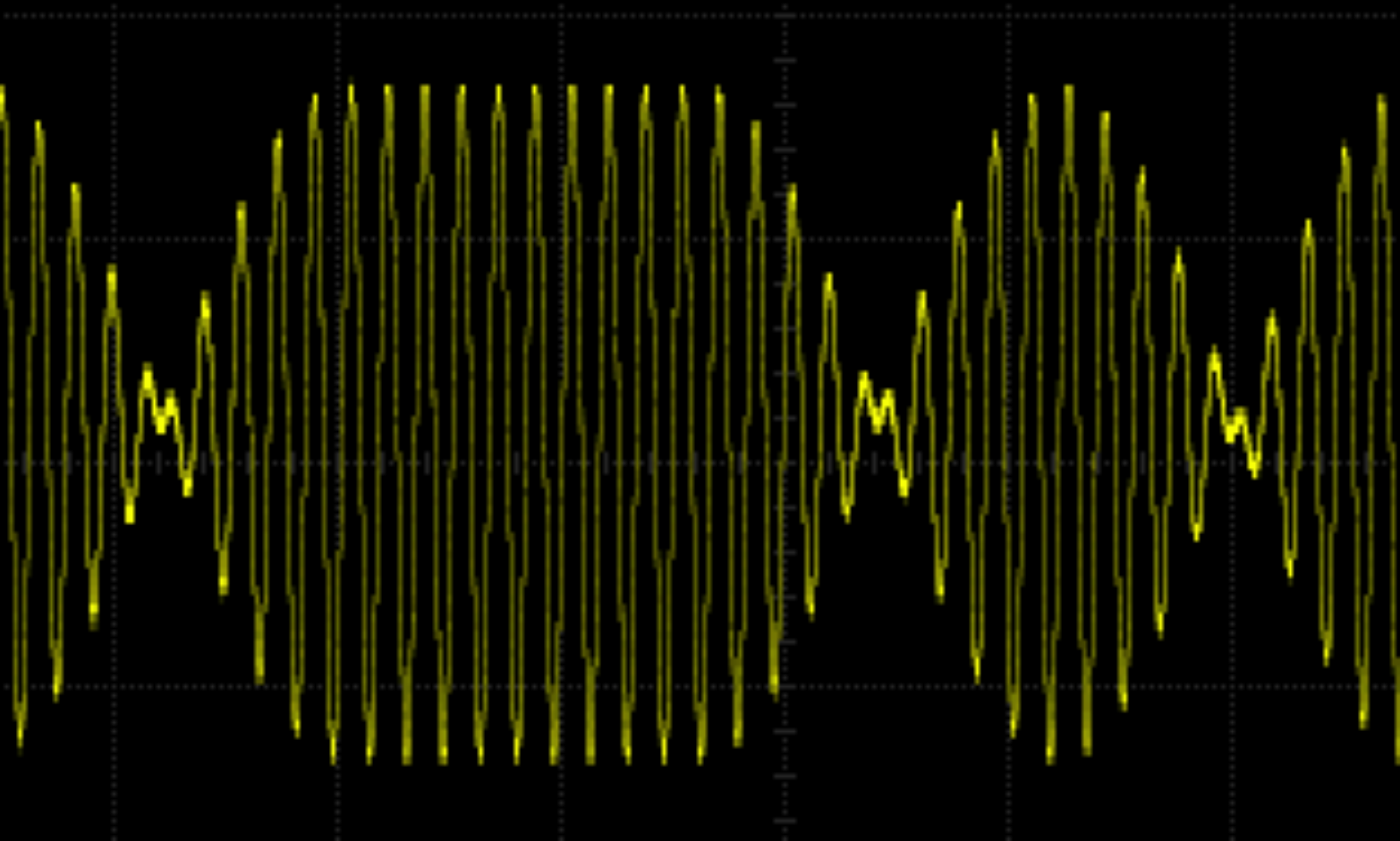
That meant I didn’t need to use the Arduino IDE and could use my code editor of choice (vim). Arduino-cli works well — thanks to the developers! BTW the Arduino IDE is fine, I’m just a terminal junkie. An oscilloscope confirmed the signal was at 50 Hz.

The picture shows me using a prototype shield on top of the Arduino. The shield is not necessary but the reset switch is easier to get at with the shield so I used it.

Did it work? Well… My turntable is a Pioneer PL-120 and the designers decided to make the speed control impossible to use while the turntable is spinning. See the yellow screwdriver which is at the speed control adjust screw in the picture of the strobe ‘disc’. So my fond dreams of shining the strobe at the disc and simultaneously adjusting the speed were dashed. I found it really difficult to do. Also it is summer here in Scotland and the weather has been good so the sun is in the sky nearly all of the time I am awake. So the LED could have been brighter to compete with the sun. It would work fine in winter or if I had better curtains.

In the end I put on a record and counted how long 10 revolutions took and did the arithmetic. Adjusted the speed (did I tell you the screwdriver is difficult to align with the speed control slot?) And repeated until good. So I didn’t actually use the strobe in the end.

A final test: ‘Oh! Wot A Dream’ by Kevin Ayers is billed as taking 2m 47s and I timed it at about 2m 46s. That’s good enough for rock and roll. Maybe someone with perfect pitch would howl in frustration — as am I waiting for the ‘Better Late…’ album.
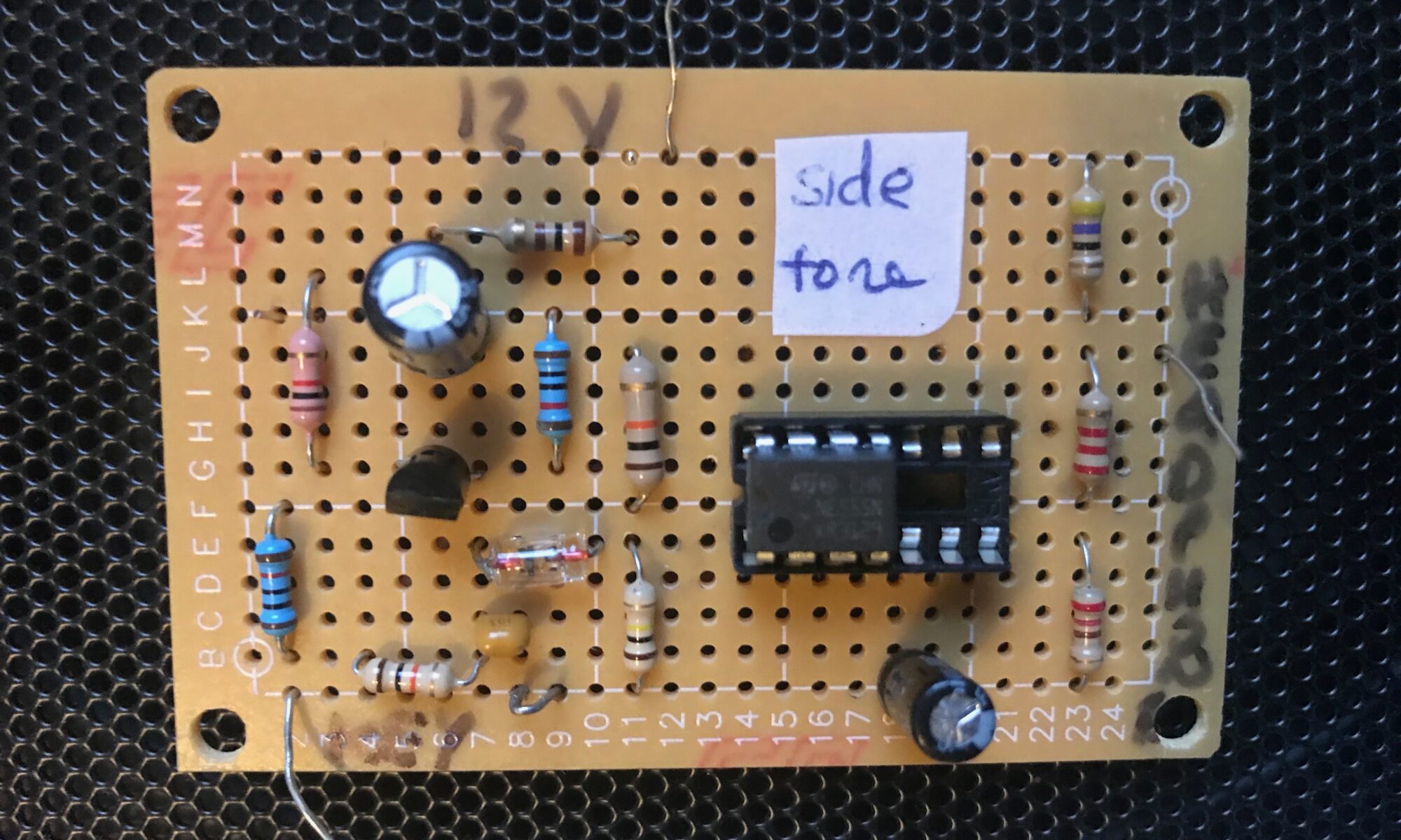
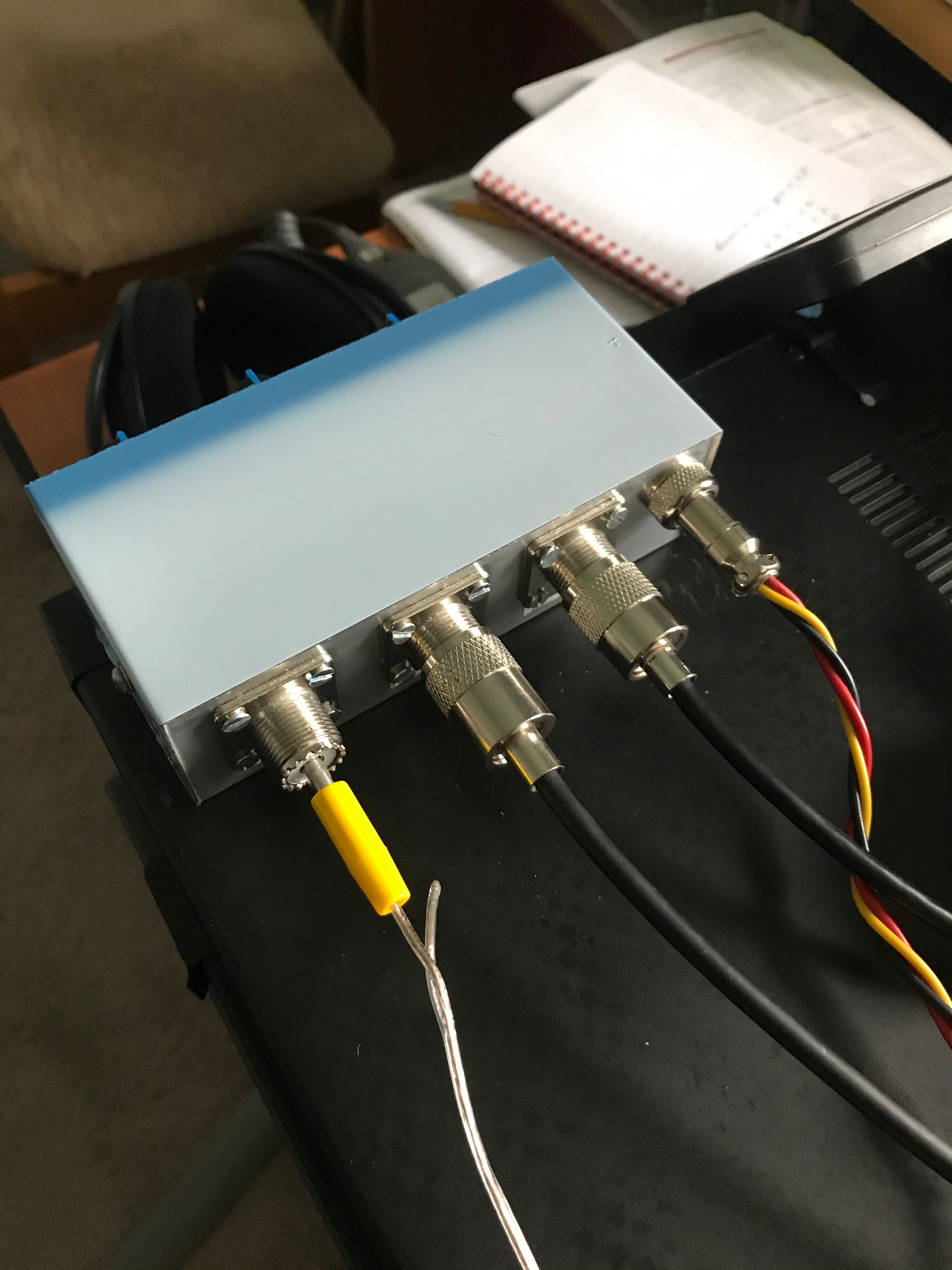
UK Deaths per Country Comparison

I thought it might be educational to compare the different health services within the UK with regard to how many COVID-19 deaths there have been, adjusted for population. Here is the result. The figures are the numbers of deaths per million population. 

Of course, each country counts deaths in its own way, so beware of how you interpret this.

The English and Scottish figures cover deaths in hospitals only and do not count deaths in care homes or people dying at home. (As at Thursday, 16 April 2020 this means the used values are 25-30% low). I believe the same is true for NI and Wales. However, it doesn’t look like the differences between the various countries would be much affected by the uncounted deaths.

The MATLAB code is here.

X-Phase — More theory

The advert is from Practical Wireless February 1987.

In my last blog I tried to explain how a QRM Eliminator works. Here’s some more information.

Suppose the signal you are trying to hear is a sine wave (shown in blue). The signal as received (shown in red) will have some noise added as it travels to you.Original noise

The QRM eliminator allows you to pick up the noise with your noise aerial and phase shift by 180º. As shown in this chart.

Noise

If you add the blue and red signal together you’d get a zero signal. So if you mix the inverted noise with the noisy signal as received you’ll recover the original signal.

Recovered

Of course reality is different and the recovered signal won’t be as clean as that. Also if you don’t match the noise and main signal amplitudes properly, you’d then get something like this.

Recovered loud

These charts were made with MATLAB using this script.

X-Phase QRM Eliminator

I bought an X-Phase QRM eliminator a while back, tried it out with a receiver and was quite impressed with its performance. It’s only recently that I’ve connected it to a transceiver because without care it is easy to damage the unit when transmitting.

QRM eliminators have been around for many years. I was recently looking at an old Practical Wireless from 1989 and S.E.M. were selling one then in the adverts at the back of the magazine. (And, yes, we used dots in abbreviations back then). If you were to be picky you might say it should be called a QRN eliminator, but it isn’t. I quite like the idea of an actual QRM eliminator though I’m not sure how you could implement it. 

Advert for QRM Eliminator

A QRM eliminator works like this: signals from the main aerial are mixed with signals from a noise aerial. The signals from the noise aerial can be shifted in phase. The idea being that you mix the main signal with the noise signal 180º out of phase. If the signals are the same you’ll just get a zero signal. But if the main signal comprises a good signal and some noise signals and the noise signal is predominantly the noise signals, you’ll end up with just the good signal. Of course, to make this work you need to be able to make the noise signals from the main and noise aerials be the same amplitude so the QRM eliminator has controls to adjust the gain of each. As you want the signals to be 180º out of phase there is also a control to adjust the phase.

front of X-Phase

The three blue knobs in the photo are these controls.

There are several QRM eliminators on the market. I got mine from Poland on eBay from the seller urbania2. The unit is solidly built in a neat aluminium box with pleasant to use control knobs and strong connexions on the back. 

The instructions are in a quaint mixture of Polish and English but I found them understandable enough as a circuit diagram is included.

I have done some quick tests on 20m with the unit and it seems to be able to reduce the background noise by about 3 S-points as shown on my TS590S transceiver. I also made some measurements using received FT8 signals. This showed an increase of about 4dB in the signal strength of CQ signals as reported by JTDX over 15 minutes with the QRM eliminator being on each even minute and off each odd minute. None of this testing was particularly scientific though. I was using a 4m length of loudspeaker wire as the noise aerial, just lying on the floor of the shack.

connexions at back of TS590S

I mentioned that it’s easy to damage the unit when transmitting. It has three wires. Red and black are for the DC supply, and the yellow wire is for the PTT. When grounded the eliminator passes the main signal straight through avoiding the damage.

This Is how I connected my TS590S. The EXT-AT connector on the TS590S provides a nominal 13.8V DC. So I used pins 1 and 6 to power the Eliminator. I got the EXT-AT plug from an eBay supplier asia_uk.

TS590S EXT AT Connection

The remote connector on the TS590S isn’t particularly well documented, but connecting the yellow wire from the Eliminator to pin 4 works, but only if menu 53 on the TS590S is set to 2. Pin 2 on the remote connector, the common terminal needs to be grounded so I connected it to pin 3 on the EXT-AT seeing it was spare. I got the required 7-pin DIN plug from RS Components.

TS590S Remote Pinouts

Graphs of coronavirus cases doubling times

I’ve added some graphs to the coronavirus cases graphs I mentioned earlier. These graphs plot how many days it takes for cases to double. So the higher the number the better.

When the peak of the cases has been reached the graphs show the number of days for the cases to halve. It does this by showing the days as negative numbers. 

I suspect that at the peak the graph will jitter quite a lot. 

I’ve suppressed the figures for the first 100 cases as the figures probably wouldn’t make any sense. Suppressed figures are set to zero.

Of course, as the governments change how they test cases the graphs will be harder to interpret.

Anyway, here’s the latest graphs. 


The MATLAB code is here.